In a nutshell
Imagine a professional kitchen at full service. A good chef never chops everything with the same knife: a paring knife for herbs, a cleaver for bone, a mandoline for wafer-thin slices. The busiest stations sit closest to the pass so plates travel the shortest distance. The chef tastes constantly instead of guessing, and when a faster oven arrives, the whole line gets re-planned around it. Performance Efficiency is running your cloud like that kitchen — pick the right tool for each job, put the work close to the diner, measure everything instead of assuming, and keep evolving as better equipment lands.
In AWS terms, “the right tool” means choosing the resource that matches how your workload actually behaves — the right compute (a virtual machine, a container, or a function), the right storage, the right database, and the right network path — and then keeping those choices efficient as traffic grows and AWS ships newer, faster options. That is the whole pillar in one sentence: use computing resources efficiently to meet your requirements, and stay efficient as demand and technology change.
Beginners sometimes hear “performance” and picture “make everything as fast as physically possible, whatever it costs.” That is not it. Performance Efficiency is about fit and evidence: the cheapest resource that comfortably meets your target, chosen because you measured it, not because it was the default your team last used. A right-sized workload is very often both faster and cheaper — on this pillar the two goals rarely fight.
Level: Advanced · Time: ~55 min read
Before you start, it helps to know:
- The AWS core building blocks — EC2 (virtual machines), S3 (object storage), EBS (disks), Lambda (functions), and a database or two (RDS/Aurora, DynamoDB). Earlier lessons in this course cover each.
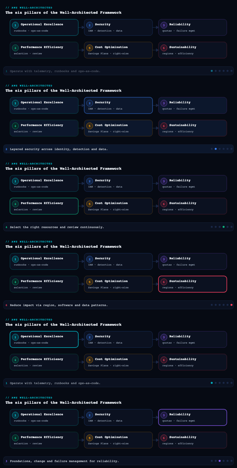
- What the Well-Architected Framework is and its six pillars. This is Part 4, the Performance Efficiency pillar, sitting between Reliability and Cost Optimization.
- The two words this whole pillar turns on: latency (how long one request takes) and throughput (how many requests you can serve per second).
After this lesson you will be able to:
- Explain the five design principles and the five best-practice areas (PERF 1–5) of the Performance Efficiency pillar in plain language.
- Select compute, storage, database, and network resources by matching them to a workload’s real access pattern instead of habit.
- Read latency at percentiles (p50/p90/p99) and write an SLO that is actually measurable.
- Design a caching hierarchy and name what each layer trades away.
- Run an AWS Well-Architected Review for this pillar and turn its findings into ranked, evidence-backed experiments.
Where this fits
Performance Efficiency is the fourth of the six pillars in the AWS Well-Architected Framework (after Operational Excellence, Security, and Reliability, and before Cost Optimization and Sustainability). Its definition is deceptively simple — use computing resources efficiently to meet requirements, and maintain that efficiency as demand changes and technologies evolve — but it is the pillar where architectural laziness costs you the most, because the cloud removes the old excuses (you can no longer claim you were stuck with the hardware procurement gave you). Its five design principles are: democratize advanced technologies (consume them as managed services rather than building them), go global in minutes, use serverless architectures, experiment more often, and consider mechanical sympathy (choose the technology that best aligns to how your workload actually behaves). The Framework expresses its expectations as five numbered best-practice questions — PERF 1 (architecture selection), PERF 2 (compute), PERF 3 (data management/storage and database), PERF 4 (networking), and PERF 5 (process and culture: review, monitoring, and trade-offs). This article walks each sub-component as you would actually implement it, naming the concrete services, artifacts, benchmarks, and trade-offs.
Architecture selection — compute, storage, database, network (PERF 1–4)
What it is. Architecture selection is the discipline of choosing, for each component of a workload, the resource type and configuration that best fits the workload’s access pattern, data shape, and performance goals — and doing so with evidence rather than habit. In a Well-Architected sense this is PERF 1 (“How do you select the appropriate cloud resources and architecture for your workload?”) decomposed across the four dimensions the cloud gives you near-infinite choice in: compute, storage, database, and network. The principle that ties them together is mechanical sympathy — matching the technology to the physics and behaviour of the workload, not to what the team last used.
Why it matters. Every other pillar inherits these choices. A latency-sensitive API placed on a throughput-optimized instance family, a random-access dataset on a throughput-optimized HDD volume, a key-value workload bolted onto a relational engine with a JOIN it was never designed for — each is a structural performance ceiling no amount of scaling or caching fully papers over. AWS publishes hundreds of instance types, half a dozen EBS volume types, multiple S3 storage classes, and more than fifteen purpose-built database engines precisely because no single resource is right for every job. Selecting well is the single highest-leverage performance decision you make, and it is cheapest to make at design time.
Compute (PERF 2)
How to do it well. Decide first which compute paradigm the workload wants — instances, containers, or functions — then optimize within it.
- Serverless first for event-driven and spiky work. AWS Lambda (with Graviton/
arm64, tuned memory, SnapStart for Java/.NET cold starts, and Provisioned Concurrency only where p99 cold-start matters) removes capacity planning entirely. Fargate gives you containers without managing nodes. Reach for these before you reach for a fleet. - Containers for steady, packable services. Amazon ECS or EKS on EC2 when you need bin-packing density, GPUs, DaemonSets, or per-second-billing nuance Fargate can’t express. Use Karpenter on EKS for just-in-time, right-sized node provisioning across many instance types.
- Instances when you need the metal. Choose the family by bottleneck: general-purpose
M, compute-optimizedC, memory-optimizedR/X, storage-optimizedI/Im4gn(NVMe), acceleratedP/G/Inf/Trn. Prefer Graviton (g-suffixed) instances — typically meaningfully better price-performance for most workloads — and validate with a benchmark rather than assuming x86 parity. - Let data choose the size. Use AWS Compute Optimizer (driven by CloudWatch + memory metrics from the agent) to surface over/under-provisioned instances, Lambda memory, ECS tasks, and EBS volumes. Treat its recommendations as a hypothesis to test, not a command.
| Workload shape | Well-suited compute | Why |
|---|---|---|
| Spiky / event-driven / unpredictable | Lambda (Graviton, SnapStart) | No idle cost, instant scale, zero capacity planning |
| Steady microservices, need density | ECS/EKS on EC2 + Karpenter | Bin-packing, fast right-sized nodes, broad instance choice |
| Stateless containers, ops-light | AWS Fargate | No node management, per-second billing |
| CPU-bound batch / encoding | C-family (Graviton c7g) + Spot |
Best compute price-performance, fault-tolerant |
| In-memory caches, big JVMs, analytics | R/X-family | High memory-to-vCPU ratio |
| ML training / inference | Trn/Inf (Neuron) or P/G (GPU) | Purpose-built accelerators beat general CPU |
Worked example: right-sizing and the Graviton decision
Selection sounds abstract until you do it with numbers, so let’s walk one decision end to end. Suppose a stateless REST service runs on 20 × m5.xlarge (x86, 4 vCPU / 16 GiB) instances. It feels fine — but is it efficient? Here is the reasoning a Well-Architected review actually follows.
Step 1 — look at the data, not the vibe. Pull two weeks of CloudWatch: average CPU sits at 22%, p95 CPU at 40%, memory at 45%, and the network is nowhere near the instance ceiling. AWS Compute Optimizer flags the fleet as over-provisioned. The bottleneck is clearly not a shortage of CPU headroom — you are paying for idle cores around the clock.
Step 2 — right-size first, then re-platform. Two independent moves are on the table, and the order matters. Right-sizing (fewer or smaller instances) captures the idle waste. Re-platforming to Graviton (arm64) captures a price-performance jump. Do the cheap, reversible move first: drop to m5.large (2 vCPU / 8 GiB) and let Auto Scaling set the count from load rather than pinning 20. That alone roughly halves the fleet with no code change.
Step 3 — benchmark Graviton, don’t assume. Now test m7g.large (Graviton3) against m5.large on the real request mix — not a synthetic CPU loop. A representative result:
| Instance | On-demand $/hr (illustrative) | Req/sec sustained at p99 < 200 ms | $ per million requests |
|---|---|---|---|
m5.large (x86) |
0.096 | 1,100 | 0.0242 |
m7g.large (Graviton3) |
0.0808 | 1,300 | 0.0173 |
Graviton is both ~16% cheaper per hour and handles ~18% more throughput at the same latency target — roughly a 28% better price-performance measured as $/million requests. That single number is what justifies the migration, and it only exists because you measured it against the workload’s own traffic. (Numbers here are illustrative — always benchmark your own mix.)
Step 4 — check the catch. Graviton runs the arm64 architecture, so container images must be multi-arch (build with docker buildx targeting linux/arm64) and any x86-native dependency — a compiled library, a monitoring agent, a licensed binary — must have an arm64 build. That is the one real migration cost; for most interpreted/JIT stacks (Go, Java, Node.js, Python, .NET) it is close to free. The full mechanics live in the Graviton migration lesson.
The takeaway pattern: measure → right-size → benchmark the alternative → quantify price-performance → verify the catch. Every compute selection in this pillar follows that loop. “We’ve always used m5” is the anti-pattern; a one-day benchmark that costs a few dollars is the cure.
Storage (PERF 3, data management)
How to do it well. Match the storage service and tier to the access pattern — sequential vs. random, latency vs. throughput, hot vs. cold, shared vs. attached.
- Object (S3). Default for static assets, data lakes, backups, and media. Choose the storage class by access frequency: S3 Standard (hot), S3 Intelligent-Tiering (unknown/changing patterns — it moves objects automatically), Standard-IA / One Zone-IA (infrequent), Glacier Instant/Flexible/Deep Archive (archival). Use S3 Transfer Acceleration or multipart uploads for large/distant transfers, and S3 Express One Zone for single-digit-millisecond, high-RPS access to hot prefixes.
- Block (EBS). For instance-attached, low-latency block storage. Default to gp3 (you provision IOPS and throughput independently of size — gp2 ties them together and is almost always the wrong default now). Use io2 Block Express for sustained high-IOPS, latency-sensitive databases; st1 (throughput HDD) for big sequential scans; never sc1 for anything random.
- File (EFS / FSx). EFS for shared POSIX access across many instances (with Infrequent Access lifecycle tiering and One Zone for cost); FSx for Lustre for HPC/ML scratch and S3-linked high-throughput; FSx for NetApp ONTAP / Windows File Server / OpenZFS for protocol-specific needs.
- Edge caching. Front S3 and APIs with Amazon CloudFront so reads are served from a Point of Presence near the user, not your origin.
| Storage need | Service / tier | Note |
|---|---|---|
| Static assets, data lake, backups | S3 (class by access) | Intelligent-Tiering when pattern is unknown |
| General DB / boot / app volume | EBS gp3 | Decouple IOPS+throughput from capacity |
| High-IOPS, latency-critical DB | EBS io2 Block Express | Sub-millisecond, consistent IOPS |
| Large sequential scans (logs, big data) | EBS st1 | Throughput-optimized HDD, not for random |
| Shared POSIX across fleet | EFS (+ IA tiering) | Elastic, multi-AZ; One Zone to save cost |
| HPC/ML high-throughput scratch | FSx for Lustre | Links to S3, hundreds of GB/s |
| Ultra-low-latency hot objects | S3 Express One Zone | Single-digit-ms, high request rate |
Database (PERF 3, data management)
How to do it well. Embrace purpose-built databases — pick the engine by data model and query pattern, not by what the org happens to standardize on. Forcing every dataset into one relational engine is the most common and most expensive Performance Efficiency anti-pattern.
- Relational: Amazon Aurora (MySQL/PostgreSQL-compatible, with Aurora Serverless v2 for variable load and Aurora I/O-Optimized for I/O-heavy workloads) or RDS. Offload reads to read replicas; for global read-locality and DR, Aurora Global Database. RDS Proxy pools connections so Lambda/serverless front-ends don’t exhaust the database.
- Key-value / document at scale: Amazon DynamoDB — single-digit-millisecond at any scale, on-demand capacity for unpredictable load, DAX for microsecond reads, and Global Tables for multi-Region active-active. Design the partition key to avoid hot partitions.
- In-memory: ElastiCache (Redis OSS / Valkey / Memcached) or MemoryDB (durable Redis) for caching and microsecond data structures.
- Search / analytics / time-series / ledger / graph: OpenSearch Service (search and log analytics), Redshift (columnar MPP warehouse, with Serverless and Spectrum over S3), Timestream (time-series/IoT), Neptune (graph), QLDB/Aurora for ledger patterns.
- Caching is an architecture choice, not an afterthought. Decide explicitly where to cache: at the edge (CloudFront), in front of the DB (DAX/ElastiCache), and in the application — and define invalidation strategy up front.
| Data / query pattern | Purpose-built service | Why |
|---|---|---|
| Transactional relational, joins | Aurora / RDS (Serverless v2, I/O-Optimized) | ACID, SQL, read replicas, managed |
| Massive key-value, predictable single-digit ms | DynamoDB (+ DAX) | Horizontal scale, on-demand, microsecond cache |
| Hot read cache / sessions | ElastiCache / MemoryDB | In-memory microsecond latency |
| Full-text search, log analytics | OpenSearch Service | Inverted index, aggregations |
| BI / data warehouse | Redshift (Serverless, Spectrum) | Columnar MPP over large datasets + S3 |
| Time-series / IoT telemetry | Timestream | Built-in tiering, time-series functions |
| Connected/graph data | Neptune | Native graph traversal |
The caching hierarchy, worked
The lesson keeps repeating “cache” — but where you cache changes everything. Think of caching as a hierarchy of shrinking, faster stores, each one catching what the layer behind it would otherwise have to recompute. Every hop you avoid is latency you never pay.
| Layer | AWS mechanism | Typical read latency | What it holds | Main trade-off |
|---|---|---|---|---|
| L0 — client | Browser cache, HTTP/CloudFront TTLs | 0 (local) | Static assets, cacheable GETs | Staleness until TTL/invalidation |
| L1 — edge | CloudFront PoP | ~10–30 ms to user | Cacheable responses, media | Cache-key design, invalidation |
| L2 — in-process | Local in-memory map | microseconds | Hot config, tiny lookups | Per-instance, lost on restart |
| L3 — shared cache | ElastiCache (Redis/Valkey), DAX | sub-ms to ~1 ms | Sessions, query results, hot items | Consistency, invalidation, cost |
| L4 — source of truth | Aurora, DynamoDB, S3 | ms and up | The truth | Slowest, most expensive per read |
Why the order pays off — do the math. Suppose the catalog-browse call costs 40 ms at the database and 1 ms from a shared cache. If the cache serves 90% of reads (a 0.9 hit ratio), the average read time is 0.9 × 1 ms + 0.1 × 40 ms = 4.9 ms — an 8× improvement from one cache layer, and the database now sees only a tenth of the traffic (so it can be smaller and cheaper too). Push the hit ratio to 0.98 and the average drops to ~1.8 ms. Hit ratio is the lever: a cache with a 40% hit ratio is mostly overhead, while the last few points near 100% deliver most of the win.
The question each layer must answer: what is the staleness budget? A cache is a copy, and a copy can be wrong. Before adding any layer, write down two things — how stale is acceptable (e.g. “catalog prices may be up to 60 s old”) and how it gets invalidated (TTL expiry, an event-driven purge on publish, or write-through). A cache without an invalidation story is a correctness bug waiting for a customer to find it. That is exactly why this pillar treats caching as an explicit trade-off, not a free speed-up.
Match the cache to the pattern. DAX sits in front of DynamoDB and speaks the DynamoDB API, so it is nearly transparent for key-value reads (microsecond item cache, write-through). ElastiCache is a general-purpose data-structure store you populate deliberately (lazy-loading or write-through). CloudFront caches at the edge, keyed by URL and cache-key policy. Reaching for the wrong one — e.g. bolting ElastiCache onto what DAX would cache transparently — adds code and bugs for no gain.
Network (PERF 4)
How to do it well. Network choices govern latency, throughput, and jitter — often the dominant term in user-perceived performance.
- Place compute near users and data. Use multiple Regions, multiple Availability Zones, Local Zones for single-digit-millisecond metro latency, Wavelength for 5G/edge, and placement groups (cluster) for low-latency, high-bandwidth inter-node traffic (HPC, distributed training).
- Pick the right instance networking. Enable Enhanced Networking (ENA), use ENA Express (SRD) for higher single-flow throughput and lower tail latency, and EFA for HPC/ML collective communication. Match the instance’s network bandwidth ceiling to the workload.
- Optimize the front door and the path. CloudFront terminates TLS at the edge and caches; AWS Global Accelerator uses the AWS backbone and anycast IPs to cut internet jitter for non-cacheable/TCP/UDP traffic; Route 53 latency- and geolocation-based routing steers users to the nearest healthy endpoint. VPC endpoints / PrivateLink keep traffic off the public internet, and Transit Gateway simplifies high-throughput inter-VPC paths.
- Choose protocols deliberately. HTTP/2 and HTTP/3 (QUIC) on CloudFront, gRPC for internal services, and connection reuse/keep-alive to amortize handshakes.
| Goal | Service / feature | Effect |
|---|---|---|
| Serve users from nearby PoP | CloudFront | Edge caching + TLS termination, lower RTT |
| Reduce jitter for dynamic/TCP/UDP | Global Accelerator | AWS backbone + anycast, faster failover |
| Route to nearest healthy endpoint | Route 53 latency/geo routing | Lower latency, regional steering |
| Metro-low-latency compute | Local Zones / Wavelength | Single-digit-ms to end users |
| High inter-node bandwidth/low tail latency | Cluster placement group + ENA Express/EFA | Tight, fast east-west traffic |
| Private, high-throughput service access | PrivateLink / VPC endpoints / TGW | Off-internet, predictable performance |
Artifacts and decisions. A documented architecture decision record (ADR) per major component capturing the chosen resource, the alternatives considered, and the data/criteria behind the choice; a benchmark harness and results (instance families, volume types, DB engines tested against the real access pattern, not a synthetic one); a caching strategy document; and a load-test report establishing baseline throughput and latency at target load. The recurring decision is evidence over inertia: run a one-day experiment (the cloud makes this nearly free) before committing a workload to a resource for years.
Performance review (PERF 5)
What it is. Performance review is the cultural and procedural mechanism for periodically re-examining your architecture against newer AWS capabilities and your own evolving requirements, then re-validating choices with benchmarks and load tests. It is the answer to “the right choice in 2024 may be the wrong choice in 2026” — AWS ships new instance families, storage tiers, and managed services constantly, and your traffic shape changes underneath you. This is the review half of PERF 5 (“How do you evolve your workload to take advantage of new releases?”).
Why it matters. Performance is not a property you set once; it is a property you sustain. Without a deliberate review cadence, workloads quietly drift into the past: still on gp2, still on x86 when Graviton would be 20–40% cheaper and faster, still on a self-managed cache that a managed service now does better. The gap compounds silently because nothing breaks — the system just costs more and runs slower than it should.
How to do it well. Run review on two clocks. A scheduled cadence (e.g., quarterly) where you conduct an AWS Well-Architected Framework Review (WAFR) using the AWS Well-Architected Tool, focused on the Performance Efficiency pillar, and triage the high-risk items (HRIs) it surfaces. And an event-driven trigger: subscribe to AWS What’s New / release notes and the Personal Health Dashboard, and when a relevant release lands (new instance generation, a new storage class, Aurora feature) you open an experiment. Make the review empirical: maintain a repeatable benchmark and load-test harness so re-validation is a button-press, not a project. Use AWS Compute Optimizer and Trusted Advisor performance checks as standing inputs, and infrastructure as code so that adopting a new instance family is a one-line, reversible change you can canary.
| Review mechanism | Tool / input | Output |
|---|---|---|
| Pillar self-assessment | Well-Architected Tool (WAFR) | Prioritized HRIs + improvement plan |
| Right-sizing signal | Compute Optimizer, Trusted Advisor | Over/under-provisioned findings |
| New-capability awareness | AWS What’s New, release notes, PHD | Candidate experiments |
| Empirical re-validation | Load-test (Distributed Load Testing on AWS) + benchmark harness | Pass/fail vs. SLO at target load |
| Pre-prod safety net | CI/CD canary + IaC | Reversible, measured rollout |
Artifacts and decisions. A completed Well-Architected Tool workload report and its improvement plan; a performance review calendar with owners; a benchmark baseline that every review re-runs; a backlog of adoption experiments tied to specific AWS releases; and an evidence trail (load-test results, before/after metrics) attached to every architecture change. The decision each cycle: which one or two changes have a high enough expected performance/cost return to justify an experiment this quarter.
Monitoring (PERF 5)
What it is. Monitoring is the continuous instrumentation that tells you whether the workload is meeting its performance goals right now, that alerts you before customers feel a regression, and that gives you the evidence to drive every other sub-component. The Framework is explicit: you should monitor performance with active (synthetic) and passive (real-user) telemetry, set thresholds tied to business goals, alarm proactively, and feed the data back into review.
Why it matters. You cannot improve, review, or make a trade-off about what you cannot see. Architecture selection without monitoring is a guess; performance review without monitoring has nothing to review. Crucially, averages lie — a healthy mean latency hides a painful p99. Monitoring at percentiles, end to end (including the network path the customer actually traverses), is what turns “it feels slow” into a precise, actionable signal.
How to do it well. Build a layered observability stack and tie every metric to a goal.
- Metrics. Amazon CloudWatch for service and custom metrics; the CloudWatch agent for memory/disk (which EC2 doesn’t emit by default); Container Insights (EKS/ECS) and Lambda Insights for the compute layer. Watch at percentiles (p50/p90/p99), not just averages, and alarm on anomaly detection rather than only static thresholds.
- Tracing. AWS X-Ray (and CloudWatch / Application Signals, OpenTelemetry-based) to find where latency accrues across distributed calls — the slow database query, the chatty downstream, the cold start.
- Synthetic (active) monitoring. CloudWatch Synthetics canaries continuously exercise critical user journeys and API endpoints from the outside, catching regressions before real users do.
- Real-user (passive) monitoring. CloudWatch RUM captures actual client-side performance (page load, Core Web Vitals) by geography and device.
- SLOs and alarms. Use CloudWatch Application Signals to define SLOs against latency/availability and burn alarms when error budget depletes. Route alarms via EventBridge/SNS to the on-call and, where safe, to auto-remediation.
- Network-layer visibility. VPC Flow Logs, ELB access logs, CloudFront logs, and Global Accelerator metrics to see the path, not just the endpoints.
| Telemetry type | AWS tool | Answers |
|---|---|---|
| Service & custom metrics | CloudWatch (+ agent) | Is each component within its threshold? |
| Compute deep metrics | Container/Lambda Insights | Where is CPU/memory/throttle pressure? |
| Distributed tracing | X-Ray / Application Signals | Which hop is adding latency? |
| Synthetic (active) | CloudWatch Synthetics canaries | Is the journey fast from the outside? |
| Real-user (passive) | CloudWatch RUM | What do real users in each region see? |
| SLO / error budget | Application Signals SLOs | Are we meeting the promise to users? |
Artifacts and decisions. A KPI / SLO catalog mapping each user-facing goal to a metric, threshold, and owner; a set of CloudWatch dashboards per service and an executive latency view; an alarm and escalation runbook; canary and RUM coverage of the top user journeys; and a performance baseline captured under known load that future comparisons measure against. The core decision is what “good” means numerically — e.g., “checkout API p99 < 300 ms at 5,000 RPS” — because an unquantified goal cannot be monitored or defended.
Trade-offs and continuous improvement (PERF 5)
What it is. This sub-component is the explicit, documented practice of acknowledging that performance is never free or absolute: you constantly trade it against consistency, durability, cost, latency, space, and time — and you keep iterating as data and technology change. The Framework calls out classic trade-offs (consistency, durability, space vs. time, latency) and pairs them with the experiment more often and evolve your workload principles. It is the synthesis of the other three: selection sets the starting point, monitoring tells you the truth, review schedules the re-think, and trade-off analysis is how you actually decide.
Why it matters. Naive “make it faster” thinking optimizes one axis and silently degrades another. Adding a cache improves latency but introduces a consistency/invalidation problem. Choosing DynamoDB eventual-consistent reads doubles read throughput per cost but may show stale data. Multi-AZ synchronous replication boosts durability but adds write latency. Precomputation trades storage for speed. A team that doesn’t make these trade-offs explicit makes them accidentally — and is then surprised when “the performance fix” causes a correctness incident.
How to do it well. Treat each trade-off as a decision with stated acceptance criteria, measured both before and after.
- Latency vs. consistency: caches (CloudFront, DAX, ElastiCache), read replicas, and eventual-consistent reads. Decide the staleness budget explicitly and document invalidation.
- Space vs. time (precompute vs. recompute): materialized views, denormalization in DynamoDB, pre-rendered/pre-aggregated data. You pay storage to buy speed — quantify both.
- Durability vs. latency: synchronous vs. asynchronous replication, write quorum settings,
fsyncbehaviour. Pick the weakest durability the use case truly tolerates, no weaker. - Cost vs. performance: Provisioned Concurrency, io2 vs. gp3, over-provisioning headroom. Set a price-performance target, not just a latency target — the cheapest way to hit an SLO usually beats the fastest-at-any-price option.
- Experiment to decide, don’t argue. Use A/B and canary deployments (CodeDeploy, feature flags), game days under synthetic load (Distributed Load Testing on AWS / Fault Injection Service for stress), and the Well-Architected Tool to track the improvement backlog. Every change carries before/after evidence from the monitoring stack.
| Trade-off axis | You gain | You give up | AWS lever |
|---|---|---|---|
| Latency vs. consistency | Speed, read scale | Freshness of data | CloudFront/DAX/ElastiCache, read replicas, eventual reads |
| Space vs. time | Faster reads/queries | Storage + write cost | Materialized views, denormalization, precompute |
| Durability vs. latency | Faster writes | Recovery guarantees | Async replication, relaxed write quorum |
| Cost vs. performance | Lower spend | Headroom / peak speed | gp3 vs io2, on-demand vs provisioned, Graviton, Spot |
| Throughput vs. ordering | Parallelism | Strict ordering | More partitions/shards (Kinesis, DynamoDB, SQS) |
Artifacts and decisions. A trade-off register (each decision: axis, choice, accepted cost, acceptance criteria, evidence); A/B / canary results; an improvement backlog in the Well-Architected Tool ranked by expected return; and a post-change performance comparison for every shipped optimization. The discipline: nothing labelled a “performance improvement” merges without naming what it trades away and proving the net result against the SLO.
Real-world enterprise scenario
StreamForge Media is a fictional video-streaming and live-events platform (~450 engineers, 18 million monthly active users across India, the EU, and the US) whose flagship app is suffering: catalog browse p99 has crept to 1.4 s, live-event start-up stalls during traffic spikes, and the analytics warehouse can’t keep up. Their VP of Engineering commissions a Performance Efficiency review aligned to the AWS Well-Architected Framework, to be delivered over two quarters. Here is what they do for each sub-component.
Architecture selection — compute. A WAFR plus Compute Optimizer reveals a fleet of over-provisioned x86 m5 instances at ~22% average CPU. They migrate stateless services to Graviton m7g/c7g on EKS with Karpenter for just-in-time right-sizing, move the spiky live-event ingest webhooks to Lambda on arm64 (with SnapStart for their Java functions), and shift fault-tolerant transcoding batch to C-family Spot. Average utilization rises to ~58%; cold-start p99 on the webhook path drops from 1.8 s to 240 ms.
Architecture selection — storage. Catalog artwork and HLS segments move to S3 with Intelligent-Tiering; the hot “now playing” segment prefixes go to S3 Express One Zone. Every gp2 volume is converted to gp3 (independently provisioning 6,000 IOPS where needed) and the metadata database moves to io2 Block Express. Origin reads drop sharply once CloudFront (HTTP/3) fronts S3 — origin egress falls ~70%.
Architecture selection — database. The “one big PostgreSQL” is decomposed by access pattern: the user session and viewing-progress store moves to DynamoDB on-demand with DAX (read p99 from 40 ms to under 2 ms) and Global Tables for multi-Region; the transactional billing core moves to Aurora PostgreSQL Serverless v2 (I/O-Optimized) with RDS Proxy in front of Lambda; catalog search moves to OpenSearch Service; and the BI workload moves to Redshift Serverless with Spectrum over the S3 data lake. ElastiCache (Valkey) caches the catalog browse response.
Architecture selection — network. Live-event and API traffic is fronted by AWS Global Accelerator (anycast over the AWS backbone) to cut jitter for non-cacheable streams; Route 53 latency-based routing steers users to the nearest of three Regions; Local Zones in Mumbai and Frankfurt shave metro latency; and inter-service east-west traffic uses PrivateLink plus a cluster placement group with ENA Express for the transcoding pipeline.
Performance review. They establish a quarterly WAFR in the Well-Architected Tool (Performance Efficiency pillar) with named HRI owners, subscribe the platform team to AWS What’s New, and stand up a repeatable load-test harness using Distributed Load Testing on AWS. Compute Optimizer and Trusted Advisor feed a standing right-sizing backlog. Adopting a new instance generation is now a one-line IaC change behind a canary.
Monitoring. They define an SLO catalog (“browse API p99 < 300 ms at 8,000 RPS”, “live start-up p95 < 2 s”) in CloudWatch Application Signals, instrument distributed tracing with X-Ray, add Container Insights and Lambda Insights, deploy CloudWatch Synthetics canaries for the top five journeys, and turn on CloudWatch RUM to see real Core Web Vitals by region. Alarms use anomaly detection and route through EventBridge to PagerDuty.
Trade-offs and continuous improvement. They keep a trade-off register: the catalog cache accepts a 60-second staleness budget (documented invalidation on publish); viewing-progress uses DynamoDB eventual-consistent reads (accepting brief staleness for 2x read throughput) but strong reads on the resume-playback call; billing keeps synchronous Aurora replication (durability over a few ms of write latency). Each optimization ships behind a canary with before/after CloudWatch evidence, and the backlog is ranked by price-performance return in the Well-Architected Tool.
Measurable outcome. Within two quarters: catalog browse p99 falls from 1.4 s to 220 ms; live-event start-up p95 from 4.1 s to 1.6 s; session-store read p99 from 40 ms to under 2 ms (DAX); fleet CPU utilization from 22% to ~58%; and compute price-performance improves roughly 35% on the Graviton-migrated tier — all while the Well-Architected Tool’s Performance Efficiency high-risk items drop from 14 to 1.
Going deeper
The core of this pillar is selection by evidence. This section is the evidence-maker’s toolkit: the small amount of math, the service internals, and the failure modes that separate a guess from an engineering decision.
The math that quietly governs performance
Two small formulas explain most performance surprises.
Little’s Law: L = λ × W, where L is the number of requests in flight (concurrency), λ is the arrival rate, and W is the average time each request spends in the system. It is not a heuristic — it is an identity, always true in steady state. That makes it a sizing tool. A service taking λ = 2,000 req/s at a mean latency of W = 50 ms must sustain L = 100 concurrent in-flight requests (2000 × 0.05). If your Lambda reserved concurrency, your RDS Proxy connection pool, or your thread count is below 100, you will queue — and no amount of extra CPU fixes a concurrency wall. Little’s Law is how you size pools and concurrency before a load test confirms it, and it explains why a slow downstream (bigger W) silently demands more concurrency at the same traffic.
Tail-latency amplification. Averages lie, and fan-out makes them lie louder. If one backend answers within its p99 target 99% of the time, a request that must wait on N independent backends is fast only when all of them are fast: P(all fast) = 0.99^N. At N = 10 that is ~90%, so the service p99 is dominated by the slowest of ten, not by any single backend’s own p99. This is why a healthy-looking microservice mesh can still feel slow, and why you monitor end-to-end percentiles, keep fan-out width honest, and consider hedged requests for the worst offenders.
Compute internals: cold starts, concurrency, and the port
A Lambda cold start is the time to create a fresh execution environment — download the code or container image, start the runtime, and run your initialization code — before the first invocation runs. It hits p99, not p50, because most invocations reuse a warm environment. Three levers, in order of preference:
- SnapStart takes an encrypted memory snapshot after init and restores it on invoke — near-zero init cost with no extra charge to keep capacity warm. It now covers Java, Python, and .NET managed runtimes. The catch: the snapshot is reused across environments, so anything that must be unique per environment (a random seed, a database connection opened at init) needs the runtime hooks to refresh it, or you get identical state everywhere.
- Provisioned Concurrency keeps N environments initialized and warm — it eliminates cold starts for that N, but you pay for the warm capacity whether it is used or not. Reserve it for the few paths where a cold-start p99 genuinely hurts users (checkout, login), not blanket across every function.
arm64(Graviton) lowers cost and latency but is orthogonal to cold starts — a warm Graviton function still needs SnapStart or Provisioned Concurrency for its cold path.
The complete cold-start playbook is its own lesson: Lambda performance — cold starts, Provisioned Concurrency, SnapStart.
Storage internals: gp3, io2, and the gp2 burst trap
The single most common storage waste is a fleet still on gp2. gp2 ties IOPS to size (3 IOPS/GiB) and hands small volumes a burst bucket: a volume under 1 TiB bursts to 3,000 IOPS by spending credits, then collapses to a low baseline when the bucket empties — a cliff that shows up as random, hard-to-explain latency spikes under sustained load. gp3 removes the coupling entirely: a flat 3,000 IOPS and 125 MiB/s baseline included, and you provision up to 16,000 IOPS / 1,000 MiB/s independently of capacity, usually at lower cost than the equivalent gp2. That is why “convert gp2 → gp3” is almost always a free win with no downtime.
For latency-critical databases, io2 Block Express provides sub-millisecond, consistent IOPS up to 256,000 IOPS / 4,000 MiB/s per volume at 99.999% durability. But mind the ceiling above the volume: every instance has an EBS-optimized bandwidth cap, so a huge io2 volume attached to a small instance is throttled by the instance, not the disk. Match all three numbers — volume IOPS, volume throughput, and instance EBS bandwidth. The tuning mechanics are covered in EBS/EFS/FSx storage performance.
Database internals: DynamoDB partitions and hot keys
DynamoDB spreads data across physical partitions by the hash of the partition key. Each partition serves roughly 3,000 read capacity units and 1,000 write capacity units per second and holds up to ~10 GB. If your access pattern hammers one key — a “celebrity” item, a monotonically increasing date bucket, a status = ACTIVE GSI that everything writes to — you get a hot partition: throttling even though the table’s total capacity looks under-used. Adaptive capacity rebalances some of this automatically by isolating frequently-accessed items, and write sharding (append a suffix 0..N to spread a hot key across N logical partitions) fixes the rest. The lesson-level anti-pattern is choosing a low-cardinality partition key; the fix is designing the key for even distribution — the heart of single-table design.
Network internals: flows, placement, and SRD
Network performance is often about a single flow, not aggregate bandwidth. Historically a single TCP/UDP flow between instances is capped (commonly 5 Gbps to most destinations, higher within a cluster placement group) even when the instance advertises 25–100 Gbps — because that headline figure assumes many parallel flows. ENA Express, built on the SRD transport (the same congestion-aware, multipath protocol behind EFA), raises single-flow throughput to up to 25 Gbps and trims tail latency, with no application changes. For HPC/ML collective communication, EFA adds OS-bypass — the kernel is out of the data path — for micro-latency all-reduce. And placement groups encode intent: cluster (one AZ, lowest latency and highest bandwidth), spread (distinct underlying hardware, max 7 instances per AZ, for small critical fleets), and partition (rack-aware, for large distributed systems such as Kafka, Cassandra, or HDFS).
Quotas, versions, and the Well-Architected Tool
Two production realities close the loop. First, Service Quotas are a performance constraint in disguise: Lambda account concurrency, per-family EC2 vCPU limits, API request rates, and EBS/EC2 throughput ceilings all cap scale — raise them before a load test, not during an incident, because some increases take time to approve. Second, the AWS Well-Architected Tool is the free, first-party home for this pillar: you answer the Performance Efficiency questions against a defined workload, it surfaces High-Risk Issues (HRIs) and Medium-Risk Issues, you save milestones to track improvement over time, and you can author custom lenses to encode your own standards. It also folds in Trusted Advisor performance checks, so the review is grounded in your actual account, not a questionnaire answered in a vacuum.
Deliverables & checklist
Common pitfalls
- Defaulting to the family you always use. Running everything on general-purpose x86 instances (or one relational engine) ignores the price-performance and fit gains of Graviton, purpose-built databases, and serverless. Fix: select by bottleneck and data shape, and validate the choice with a one-day benchmark before committing.
- Optimizing on averages, then being blindsided by p99. A healthy mean latency routinely hides a tail that drives churn. Fix: define and alarm on percentile-based SLOs (p90/p99), and add synthetic + real-user monitoring so you see the outside-in experience.
- Treating storage tier and volume type as set-and-forget. Leftover
gp2volumes, S3 Standard for cold data, and uncached read paths quietly cost speed and money. Fix: standardize on gp3, use S3 Intelligent-Tiering for unknown patterns, and front read-heavy paths with CloudFront/DAX/ElastiCache. - Adding a cache without owning invalidation. Bolting on a cache to “make it faster” introduces a consistency bug if staleness and invalidation aren’t designed. Fix: record the staleness budget and invalidation strategy in the trade-off register, and use strong reads only where correctness demands them.
- Selecting once and never reviewing. The cloud ships better options constantly; a workload that’s never re-evaluated drifts into the slow, expensive past. Fix: run a quarterly Well-Architected review, subscribe to AWS releases, and keep adoption a reversible, IaC-driven experiment.
- Calling something a “performance improvement” with no evidence. Changes shipped on intuition can regress cost, durability, or a different latency path. Fix: require before/after monitoring data and a named trade-off for every optimization, validated behind a canary.
Practice challenges
Work these in order — they escalate from beginner to advanced. Try each before opening the solution.
1. (Beginner) Name the design principle. For each choice, name which of the five Performance Efficiency design principles it illustrates: (a) using Amazon Aurora instead of running your own MySQL on EC2; (b) deploying to three Regions in an afternoon to serve a new continent; © spinning up a one-day benchmark of two instance families before committing; (d) choosing a memory-optimized R-family instance because the workload is a large in-memory cache; (e) replacing a cron-on-EC2 job with an event-driven Lambda.
<details><summary>Solution</summary>
(a) Democratize advanced technologies (consume a managed service instead of building it). (b) Go global in minutes. © Experiment more often. (d) Mechanical sympathy (match the technology to how the workload behaves). (e) Use serverless architectures.
Why: the five principles are the vocabulary this pillar reasons in — mapping real choices back to them is the first skill a reviewer needs. </details>
2. (Beginner) Pick the storage. Choose the best storage service/tier for: (a) 4 KB thumbnails read constantly by a global audience; (b) compliance logs kept 7 years and read maybe once; © a PostgreSQL data volume that needs a steady 8,000 IOPS; (d) a shared POSIX directory mounted by 30 instances; (e) HLS “now playing” segments needing single-digit-millisecond reads at very high request rates.
<details><summary>Solution</summary>
(a) S3 Standard behind CloudFront. (b) S3 Glacier Deep Archive. © EBS gp3 with 8,000 IOPS provisioned. (d) Amazon EFS. (e) S3 Express One Zone.
Why: storage fit is access-pattern matching — frequency, sharing model, latency target, and IOPS decide the answer, not habit. </details>
3. (Intermediate) Cache math. A read costs 25 ms at the database and 1 ms from ElastiCache. (a) If the cache hit ratio is 0.8, what is the average read latency? (b) What hit ratio do you need to bring the average under 3 ms?
<details><summary>Solution</summary>
(a) 0.8 × 1 + 0.2 × 25 = 0.8 + 5 = 5.8 ms. (b) Solve h × 1 + (1 − h) × 25 ≤ 3 → 25 − 24h ≤ 3 → 24h ≥ 22 → h ≥ 0.9167, so you need roughly a 92% hit ratio.
Why: the hit ratio, not the mere presence of a cache, is the lever — and the gains that matter most sit in the last few points near 100%. </details>
4. (Intermediate) Purpose-built database. Choose the engine for: (a) a shopping-cart/session store, single-digit-ms, massive scale; (b) full-text product search with typo tolerance and facets; © BI dashboards scanning billions of rows; (d) 12 months of device-telemetry time series; (e) transactional billing needing ACID and SQL joins.
<details><summary>Solution</summary>
(a) DynamoDB (with DAX for microsecond reads). (b) OpenSearch Service. © Redshift (Serverless / Spectrum). (d) Timestream. (e) Aurora / RDS.
Why: “one relational engine for everything” is the classic and most expensive anti-pattern — match the data model and query pattern to a purpose-built engine. </details>
5. (Advanced) Little’s Law. A service receives 3,000 req/s at a mean latency of 40 ms. (a) How many requests are in flight (concurrency)? (b) Your Lambda reserved concurrency is 100 — what happens? © A new downstream raises mean latency to 120 ms at the same rate — what is the new required concurrency?
<details><summary>Solution</summary>
(a) L = λ × W = 3000 × 0.040 = 120 in flight. (b) 100 < 120, so requests queue and throttle — a concurrency wall that extra CPU cannot fix; raise reserved concurrency (and the account quota) to ≥ 120 with headroom. © L = 3000 × 0.120 = 360 — a 3× jump in required concurrency purely from the slower downstream.
Why: concurrency equals arrival-rate × latency; pools and Lambda concurrency must be sized to it, and a slow dependency silently blows the budget. </details>
6. (Advanced) Trade-off register entry. You want to cache the catalog-browse response to cut p99. Write the trade-off register entry: axis, choice, accepted cost, acceptance criteria, evidence, and invalidation.
<details><summary>Solution (one valid answer)</summary>
- Axis: latency vs. consistency.
- Choice: ElastiCache (Valkey) in front of Aurora for the browse response.
- Accepted cost: up to 60 s staleness on price/inventory in the browse view.
- Acceptance criteria: browse p99 < 300 ms at 8,000 RPS and zero stale-price checkout incidents.
- Evidence: before/after CloudWatch p99 plus a load test at 8,000 RPS, shipped behind a canary.
- Invalidation: event-driven purge on catalog publish, with a 60 s TTL backstop; the checkout path uses a strong read from the source, never the cache.
Why: on this pillar a “performance improvement” is not done until it names what it trades away and proves the net result against an SLO — that is the whole discipline in one artifact. </details>
Common beginner mistakes
These are conceptual traps — wrong mental models — distinct from the operational pitfalls listed earlier.
- “Performance Efficiency means making everything as fast as possible.” No — it means efficiently meeting a stated requirement. The target is an SLO, and the cheapest resource that comfortably meets it wins. Over-provisioning for speed nobody asked for is itself a form of inefficiency this pillar warns against.
- “Serverless is always faster and cheaper.” Serverless removes capacity planning and shines for spiky, event-driven work — but a steady high-throughput service can be cheaper on right-sized containers or instances, and cold starts can hurt p99. Choose by workload shape, not by slogan.
- “A bigger instance / more vCPUs is always faster.” Throughput scales with the bottleneck resource, not the vCPU count. A memory-bound, I/O-bound, or single-threaded workload gets nothing from extra cores. Profile to find the real bottleneck first, then size for it.
- “The average latency looks great, so users are happy.” Users feel the tail. A 50 ms average can hide a 900 ms p99 that drives churn, and fan-out amplifies tails. Set and alarm on percentile SLOs (p90/p99) and add real-user monitoring so you see the outside-in experience.
- “A cache is a free speed-up.” A cache is a copy, and every copy can go stale. You are trading consistency for latency; without a staleness budget and an invalidation plan you have swapped a slow-but-correct system for a fast-but-wrong one.
- “Graviton is just a cheaper x86 — flip a switch.” Graviton is the
arm64architecture. You need multi-arch images andarm64builds of any native dependency. For most managed/interpreted stacks it is near-free, but verify with a benchmark and check your dependencies rather than assuming binary compatibility. - “We chose the right architecture, so we’re done.” The right choice in 2024 is often wrong by 2026 — AWS ships faster options constantly and your traffic changes underneath you. Performance Efficiency is a loop (review → benchmark → evolve), not a one-time decision. No review cadence means silent drift into the slow, expensive past.
Glossary
- Performance Efficiency pillar — the Well-Architected pillar about using computing resources efficiently to meet requirements and staying efficient as demand and technology change.
- Design principles (the five) — democratize advanced technologies, go global in minutes, use serverless architectures, experiment more often, and consider mechanical sympathy.
- Mechanical sympathy — choosing the technology that best aligns with how the workload actually behaves (its access pattern, data shape, and physics), not with team habit.
- PERF 1–5 — the pillar’s five best-practice questions: architecture selection (1), compute (2), data management/storage & database (3), networking (4), and process/culture — review, monitoring, trade-offs (5).
- WAFR — Well-Architected Framework Review: a structured self-assessment of a workload against a pillar’s questions.
- AWS Well-Architected Tool — the free, first-party service where you run a WAFR, receive risk findings, save milestones, and apply custom lenses.
- HRI / MRI — High-Risk Issue / Medium-Risk Issue: the prioritized findings the Well-Architected Tool surfaces.
- Latency — how long a single request takes (measure it at percentiles, not just the mean).
- Throughput — how many requests or how much data you process per unit time (e.g. RPS, MiB/s).
- IOPS — input/output operations per second; the count of discrete reads/writes a storage volume sustains (distinct from throughput, which is bytes/sec).
- Percentile (p50/p90/p99) — the value below which that fraction of samples fall; p99 latency is the experience of the slowest 1% and is what tail-sensitive users feel.
- SLO / SLI / error budget — the target (Objective) on a measured Indicator, and the allowable amount of missing it before you must stop shipping risk.
- Little’s Law —
L = λ × W: concurrency equals arrival rate times average time-in-system; the identity used to size pools and concurrency. - Graviton / arm64 — AWS’s Arm-based processors (e.g.
m7g,c7g); typically better price-performance, but requirearm64builds. - Right-sizing — adjusting instance/function/volume size to match measured demand, removing idle waste.
- AWS Compute Optimizer — a service that analyzes CloudWatch metrics to flag over- and under-provisioned EC2, ASGs, Lambda, ECS-on-Fargate, and EBS.
- Instance family — a group of instance types tuned to a bottleneck:
Mgeneral,Ccompute,R/Xmemory,Istorage,P/G/Inf/Trnaccelerated. - Cold start — the one-time cost of initializing a new Lambda execution environment before its first invocation; hits p99.
- SnapStart — Lambda feature that restores a post-init memory snapshot to cut cold starts (Java, Python, .NET) at no extra warm-capacity charge.
- Provisioned Concurrency — pre-initialized, always-warm Lambda environments that remove cold starts for a set count, at the cost of paying for that capacity.
- EBS gp3 — general-purpose SSD volume where IOPS and throughput are provisioned independently of size (3,000 IOPS / 125 MiB/s baseline included).
- EBS io2 Block Express — high-end SSD for latency-critical databases: sub-ms, consistent IOPS up to 256,000, 99.999% durability.
- Burst bucket (gp2) — the credit mechanism that lets a small gp2 volume burst to 3,000 IOPS, then collapse when credits run out — a common latency-spike source.
- S3 storage class — S3 tier chosen by access frequency: Standard, Intelligent-Tiering, Standard-IA/One Zone-IA, Glacier Instant/Flexible/Deep Archive.
- S3 Intelligent-Tiering — an S3 class that moves objects between access tiers automatically when the pattern is unknown or changing.
- S3 Express One Zone — a single-AZ, single-digit-millisecond, high-RPS S3 class for hot data (directory buckets).
- Purpose-built database — using the engine that fits the data model/query pattern (relational, key-value, in-memory, search, warehouse, time-series, graph) instead of forcing one engine.
- Partition key / hot partition — the DynamoDB attribute that decides data placement; a low-cardinality or overloaded key concentrates traffic on one partition and throttles.
- Adaptive capacity — DynamoDB’s automatic rebalancing that isolates frequently-accessed items to relieve hot partitions.
- DAX — DynamoDB Accelerator: an in-front, write-through cache giving microsecond reads via the DynamoDB API.
- Read replica — a read-only copy of a database that offloads read traffic from the primary.
- Aurora Serverless v2 — Aurora capacity that scales in fine-grained ACUs to match variable load.
- RDS Proxy — a managed connection pool that keeps serverless/Lambda front-ends from exhausting database connections and speeds failover.
- ElastiCache — managed in-memory cache (Redis/Valkey/Memcached) for sessions, query results, and hot items.
- Caching hierarchy / hit ratio — the ordered layers of caches (client → edge → in-process → shared → source) and the fraction of reads a layer serves.
- Staleness budget — the maximum acceptable age of cached data, decided and documented before adding a cache.
- Invalidation — how a cache entry is refreshed or purged (TTL expiry, event-driven purge, write-through) to bound staleness.
- Placement group — an EC2 placement strategy: cluster (low latency, one AZ), spread (distinct hardware), partition (rack-aware for large distributed systems).
- ENA / ENA Express / SRD — Elastic Network Adapter; ENA Express uses the SRD transport to raise single-flow throughput (up to 25 Gbps) and cut tail latency.
- EFA — Elastic Fabric Adapter: OS-bypass networking for HPC/ML collective communication.
- AWS Global Accelerator — anycast IPs over the AWS backbone that reduce internet jitter for non-cacheable TCP/UDP traffic and speed failover.
- CloudFront / PoP / anycast — the CDN that caches and terminates TLS at edge Points of Presence; anycast routes users to the nearest one.
- Route 53 latency-based routing — DNS routing that steers each user to the Region giving them the lowest measured latency.
- Local Zones / Wavelength — AWS infrastructure placed in metros / telco 5G networks for single-digit-millisecond latency to nearby users.
- PrivateLink / VPC endpoint — private, off-internet access to AWS or partner services for predictable performance and security.
- Service Quotas — the account/Region limits (concurrency, vCPUs, request rates) that cap scale and must be raised ahead of load tests.
- Canary deployment — releasing a change to a small slice of traffic first, with before/after metrics, so a regression is caught and rolled back cheaply.
- Trade-off register — the artifact recording each performance decision: axis, choice, accepted cost, acceptance criteria, and evidence.
What’s next
Part 5 of the AWS Well-Architected Framework series turns to the Cost Optimization pillar — practicing cloud financial management, expenditure and usage awareness, selecting cost-effective resources, managing supply against demand, and optimizing over time.